Disclosure: I am short SPY.
In a recent article
we explored some optimizations of a simple way to trade the S&P
500. In this article we'll take one additional step in developing a
higher performance strategy to trade SPY that's still easy to implement.We'll begin with an observation; this is not your father's or grandfather's market. We've gone from fractional values for shares to decimal and now we even have high frequency traders competing for fractions of fractions and a market that trades in microseconds. What's really been striking over the last 7-10 years in the markets is the explosive growth and proliferation of ETFs. Of particular interest are the original index centric ETFs that purport to accurately mimic the behavior of popular indexes like the S&P 500 (SPY) in 1993, the Dow Jones Industrial Average (DIA) in 1998, the NASDAQ 100 (QQQ) in 1999, and the Russell 2000 (IWM) in 2000 to name a few. What is even more interesting from a modeling and trading perspective was the introduction of inverse ETFs for each of these indexes that purport to accurately mimic shorting an index; these include (SH), (DOG), and (PSQ) in 2006, and (RWM) in 2007. For now we'll assume that, at least for short periods of time, these inverse ETFs do what they claim and reflect a true short position in their respective indexes to a reasonable degree of accuracy (they don't but the differences can be small for short time periods).
Let's start with a short review of the original strategy presented in a previous article, and the optimization proposed in the most recent article. The original strategy was a simple "skimming" algorithm; simply stated the strategy is you are long the S&P 500 when the price of the S&P 500 is above its 300-day Simple Moving Average [SMA], and you retreat to cash when the price is below the 300-day SMA. This is easily modeled using a spreadsheet and the results were a bit disappointing when viewed over the 20-year price history for the SPY ETF.
(click to enlarge)
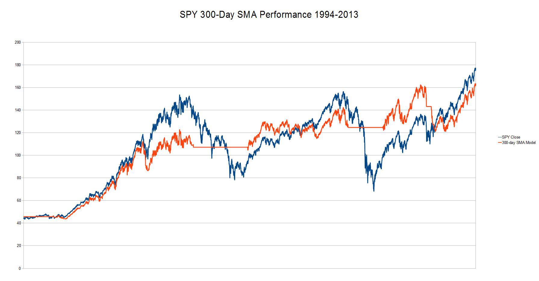
Performance Ratio = 0.91:1
The most recent article improved on this strategy by first optimizing the value of the SMA chosen to produce an optimal result for the 20-year period, and then by employing a leveraged ETF (SSO) to further increase overall gain. For this article we'll leave the leveraged ETFs out; my basic tenet is if you can get a model to work well with unleveraged ETFs then using leveraged ETFs will probably add both volatility and gain although you'll likely not see anywhere near the 2X gain they advertise. For this article all runs will be done close to close; i.e., the switch from long to cash or long to short will be done at the market close on the day the transition occurs.
(click to enlarge)
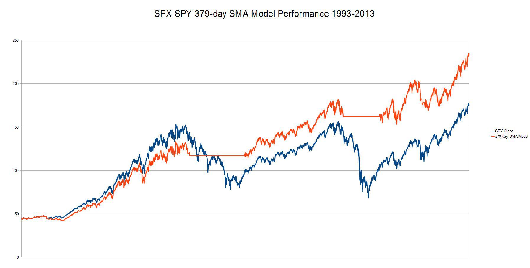
Performance Ratio = 1.35:1
So let's look a bit at algorithms, trading strategies and models. From our experience the basic idea is to look for an edge that persists over time and also works on multiple indexes and asset classes. Generally, the longer the time frame that's used in generating the model the better, but probably just as important is that the time frame chosen include at least 2 bull markets and 2 corrections to have some degree of confidence, going forward, that the model will continue to accurately follow the index and outperform whatever baseline you choose. Typically the baseline or benchmark is a simple buy and hold strategy in the underlying index.
A trading algorithm can take many forms and have a wide range of rules from simple to complex, but in the case of trying to beat an index the key metric is simply the performance ratio achieved. We define that as the total gain over a given time frame that the algorithm delivers divided by the total gain that a simple buy and hold strategy would deliver. The original and optimized algorithms in the earlier articles are what I call "skimming" algorithms, they're either 100% Long or 100% Cash, never Short. If you think about that you'll quickly realize the following:
- When the algorithm is long the best you can do is simply track the underlying index. If the index goes up 1% you gain 1% and if the index goes down 1% you lose 1% (assuming there's negligible slippage in the ETF), but you cannot gain a performance advantage over the underlying index.
- When the algorithm is in cash, this is the only opportunity in a skimming algorithm to gain a performance advantage over the index. If the index goes down 1% and the algorithm has you in cash, you effectively gain a 1% advantage over the index. Conversely, if the index goes up 1% and you're in cash you effectively lose 1% relative to the index.
- Last, we'll introduce the ability, via inverse ETFs beginning in 2006/2007 to go short the index using a timing algorithm. In this case we're essentially "supercharging" a cash position; if the index goes down 1% and we're short presumably we'll gain 1% resulting in a 2% performance advantage. However, like all things in the market there's no free lunch. If the algorithm is wrong, and the index goes up 1% we'll lose 1% and effectively lose 2% relative to the index.
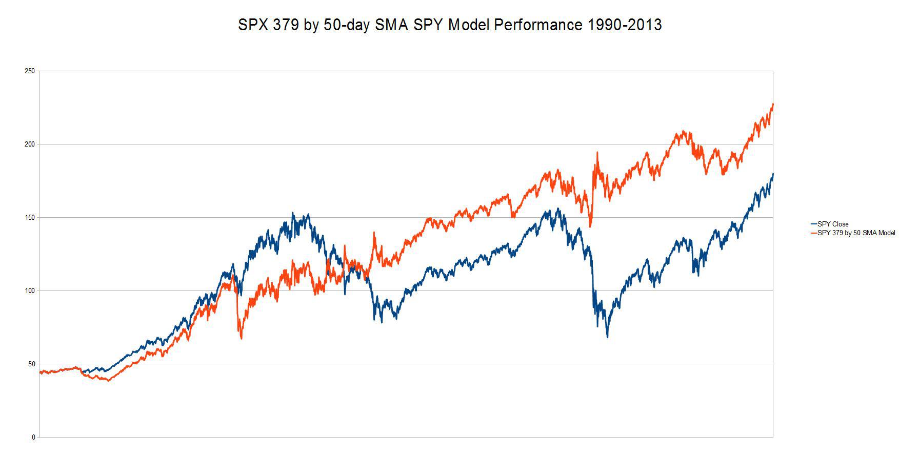
To begin, we'll simply take our optimized 379-day SMA strategy and go short instead of cash when the price of the S&P 500 is below its 379-day SMA.
(click to enlarge)
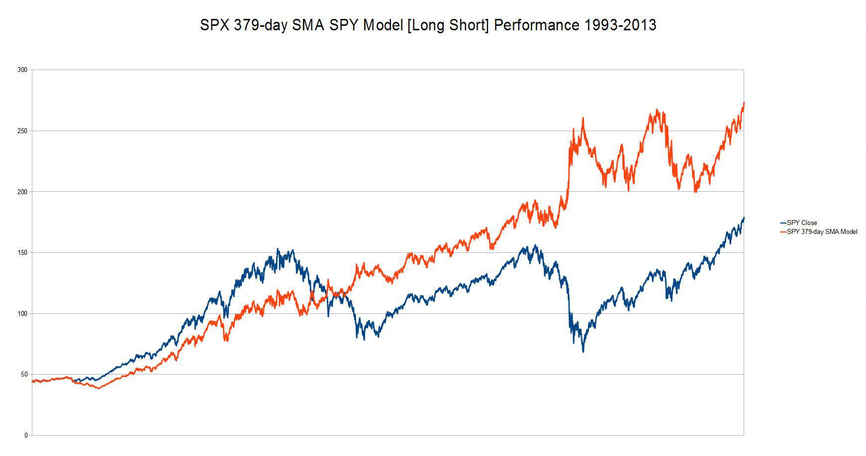
Performance Ratio = 1.53:1
We now have a somewhat higher performance ratio versus moving to cash, but what is also quickly apparent is that the algorithm produces a pretty volatile chart with a significant drawn down in the 2009-2011 region. So is there a way to improve on this, substantially reduce the volatility, and retain or improve performance?
Let's look at the 379-day SMA chart vs the S&P 500 and a couple of data points.
(click to enlarge)
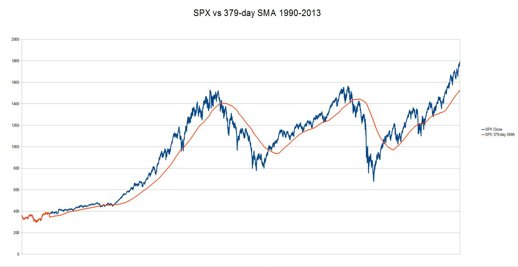
It's clear from a simple visual inspection that we have three peaks and two valley in the chart; what's also clear is that the 379-day SMA algorithm does a pretty decent job of getting into cash or short near a peak, but a pretty poor job of getting back to long near a bottom. Here's a couple of data points to illustrate:
2000 Peak 9/01/2000 1520.77
2000 379-SMA Crossover 10/10/2000 1387.02
Lag = 133.75 (8.8%)
2003 Valley 3/11/2003 800.73
2003 379-SMA Crossover 6/4/2003 986.24
Lag = 185.51 (23.2%)
2007 Peak 10/09/2007 1565.15
2008 379-SMA Crossover 1/4/2008 1411.63
Lag = 153.52 (9.8%)
2009 Valley 3/09/2009 676.53
2009 379-SMA Crossover 9/14/2009 1049.34
Lag = 372.81 (55.1%)
What we observe here is that while the lag from the peak to a crossing of the 379-day SMA from above is under 10%, the lag from a bottom to a crossing of the 379-day SMA from below is much larger. How do we fix this? One way is to look for a shorter duration SMA for the short side.
(click to enlarge)

This chart shows both a 379-day SMA and a popular SMA for trading algorithms, the 50-day SMA.
So here's the algorithm we'll initially look at:
When the price of the S&P 500 (SPX) is above its 379-day SMA the algorithm is Long.
When the price of SPX is below its 379-day SMA then:
- if the price of the SPX is below its 50-day SMA then the algorithm is Short
- if the price of the SPX is above its 50-day SMA then the algorithm is Long
(click to enlarge)
Performance Ratio = 1.26:1
So comparing this chart to the previous 379-day SMA Long Short Chart we've clearly reduced volatility but also sacrificed a lot of overall gain as we now have a lower Performance Ratio. So let's do some optimization on the short duration SMA (50-day) to see if we can find a set of better, optimal values. We'll write a little code and look at a range of both long duration and short duration SMAs in combination. We'll sweep from a long duration SMA of 375 to 425 and a short duration SMA from 50 to 100.
(click to enlarge)

It turns out that there's two combinations that produce the same peak value:
Long Duration = 393 or 394 SMA
Short Duration = 77 SMA
What I believe is also important is that the Percent Gain chart is fairly consistent; there's a wide range of values that produce a decent gain (say > 200%) although the algorithm is sensitive to the low duration SMA. Next, let's look at the performance graph of 393 SMA by 77 SMA.
(click to enlarge)
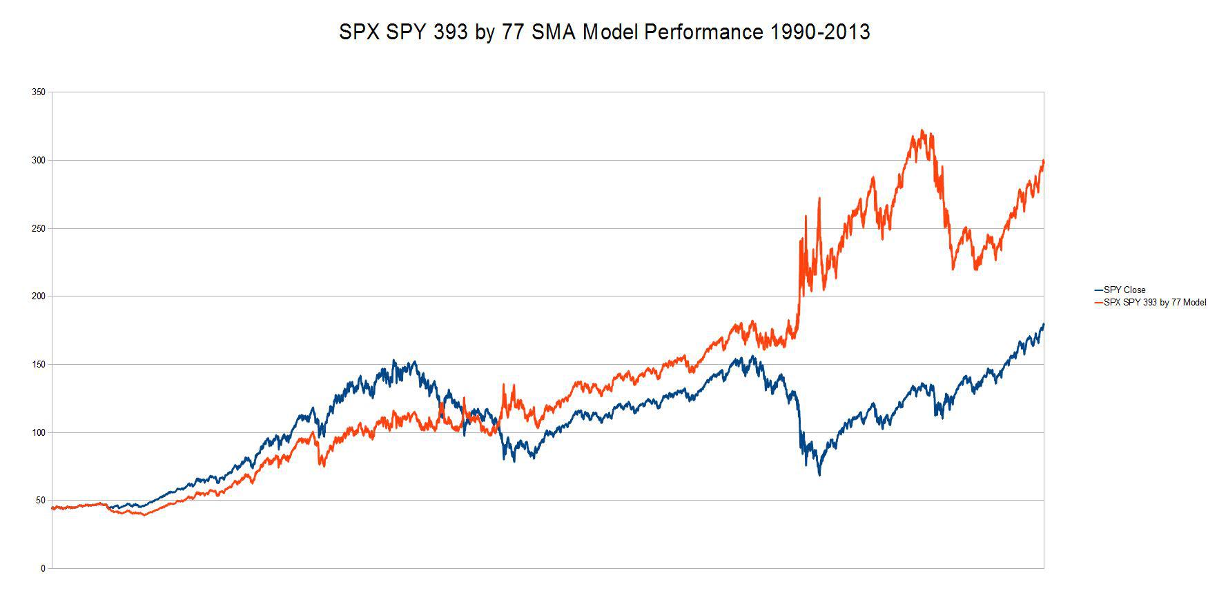
Performance Ratio = 1.66:1
So we now have more performance but at a cost of rather high volatility, especially in the 2011 region. There's one more "tweak" we can look at: instead of executing the transition when the price is below the long duration SMA (393) based on price moving up above a short duration SMA (77) let's look at using the slope (positive versus negative) of a short duration SMA to toggle the transition between short and long.
First, we'll need to sweep across SMA pairs using this new rule to find an optimal pair. For this study we'll sweep from a long duration SMA from 375 to 425 and a short duration SMA from 2 to 20.
(click to enlarge)
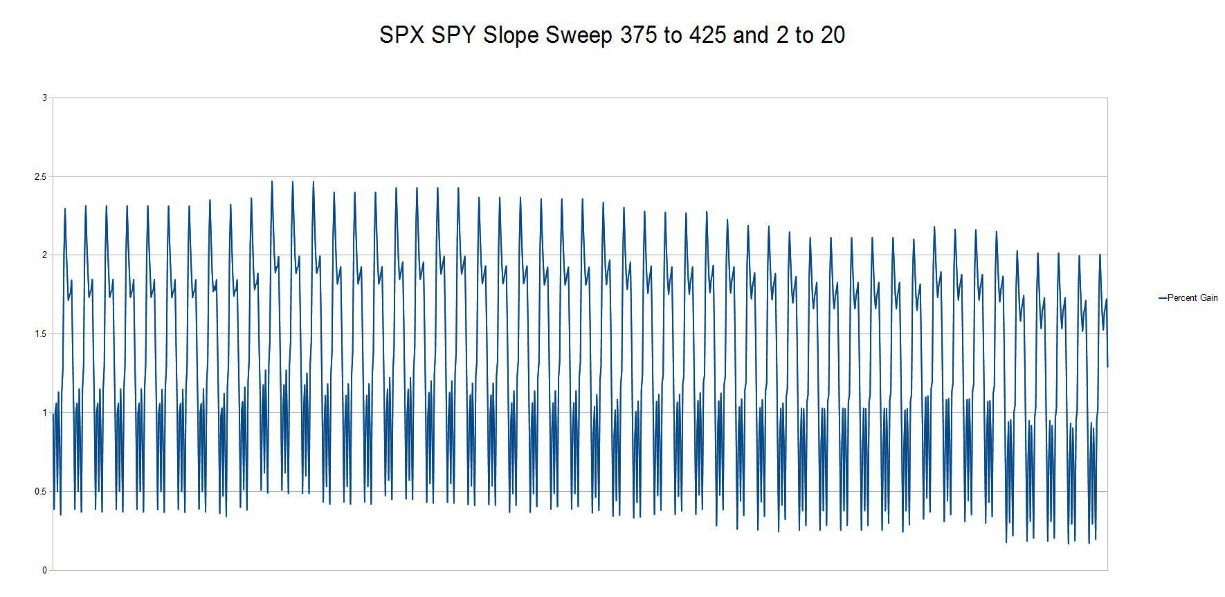
For this new algorithm, using the slope of a short duration SMA to transition from short back to long, the optimal values are 385 for the long duration SMA and 13 for the short duration SMA. The performance graph for this combination looks like this:
(click to enlarge)
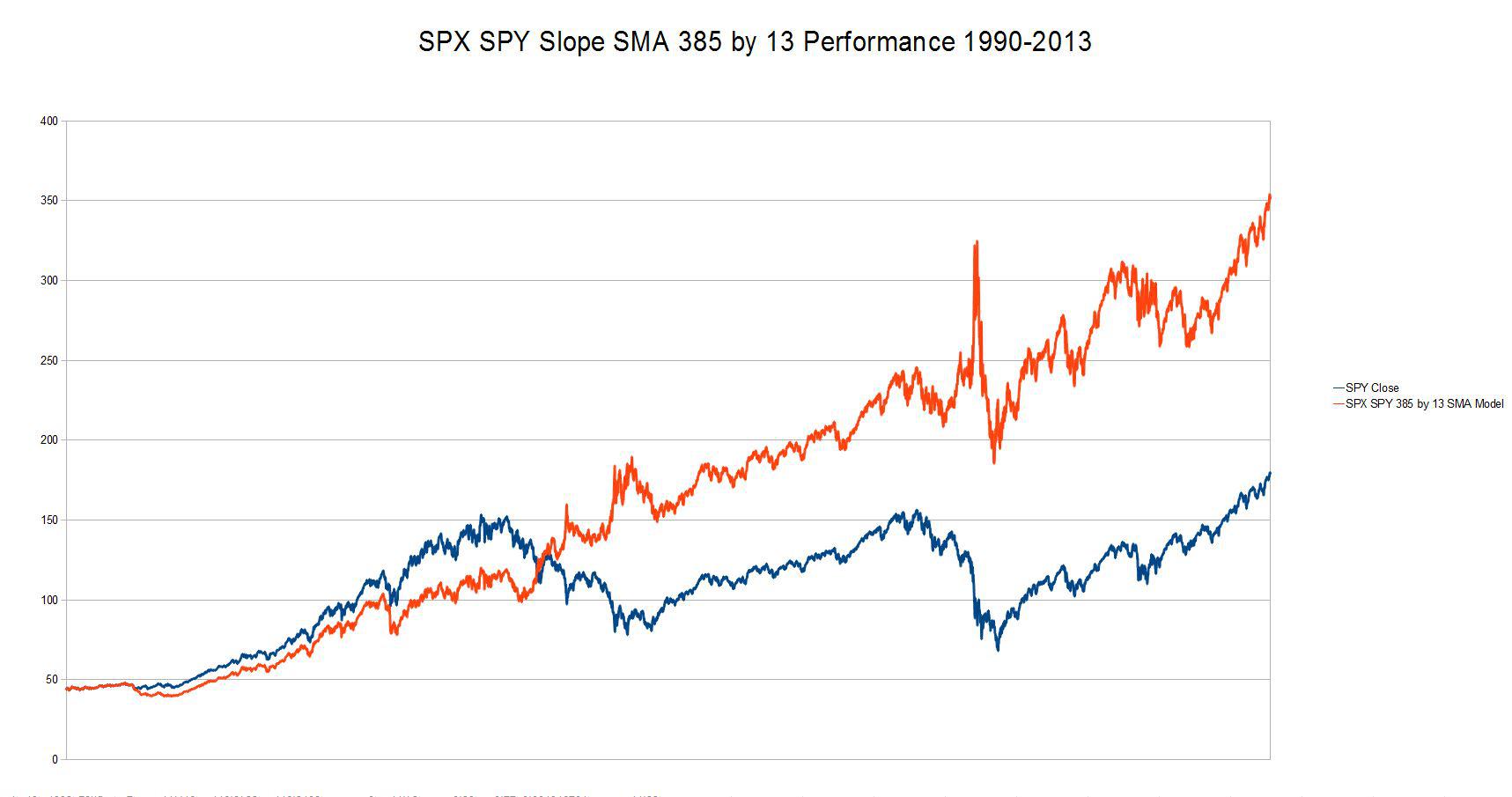
Performance Ratio 1.96:1
So now we've got a really nice performance ratio (nearly 2:1) with some volatility, especially in the 2008-9 downturn but overall a decent chart.
Last, I know I'll get questions about dividends. So here's a final chart of the SPX SPY 385 by 13 Slope SMA Model where the baseline is now the "Adjusted Closing Price" for SPY and we've accounted for the dividends when the model is Long.
(click to enlarge)
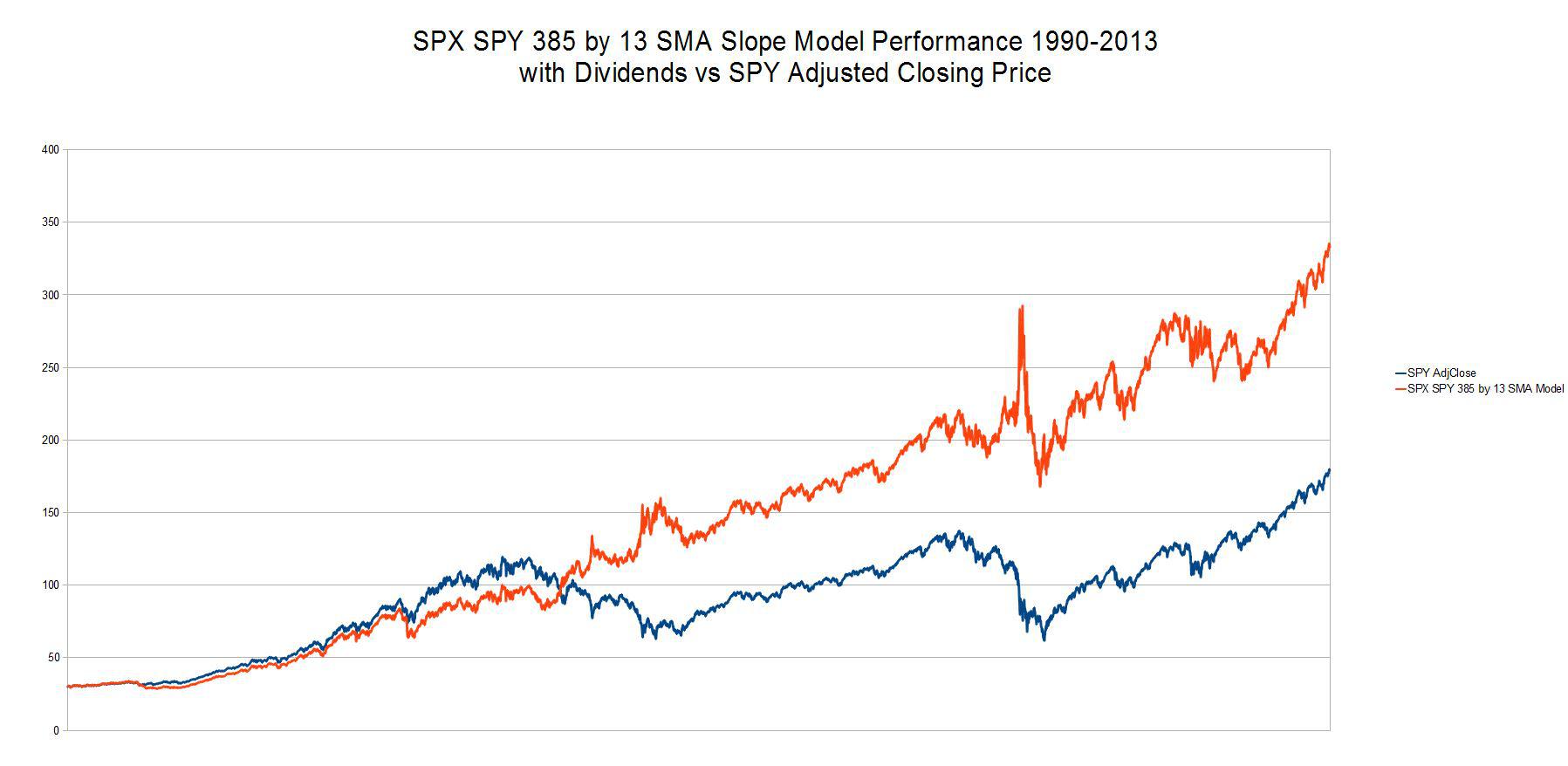
Performance Ratio 1.86:1
No comments:
Post a Comment