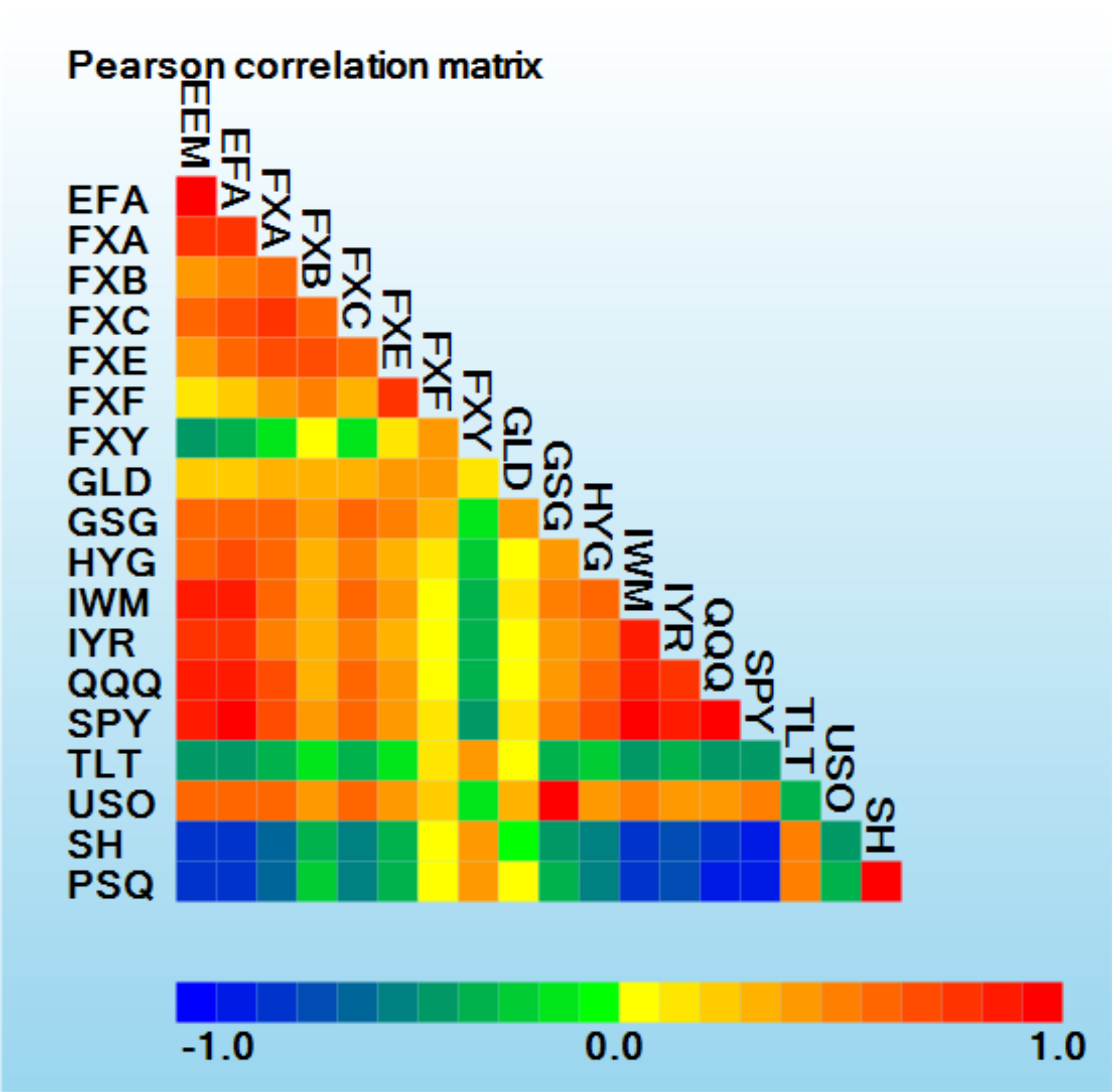
Portfolio managers periodically assess the performance of asset-preserving or hedging portfolios comprised of assets that are typically less risky than high-return assets, in order to prepare for periods of prolonged instability or deep market corrections. To evaluate several current possibilities, portfolios rebalanced on a quarterly basis were generated using a variety of techniques to determine the stability in returns. A heat map of 6-year correlation coefficients is shown below for a basket of "collar" type hedging assets. As usual, the Japanese Yen (
FXY) has not correlated with the majority of other currencies. This is also evident for long-term treasuries (
TLT), shorting ETF (
SH) for the S&P 500 Index, and shorting ETF (
PSQ) for the NASDAQ-100 Index.

Using the correlation matrix
R and covariance matrix
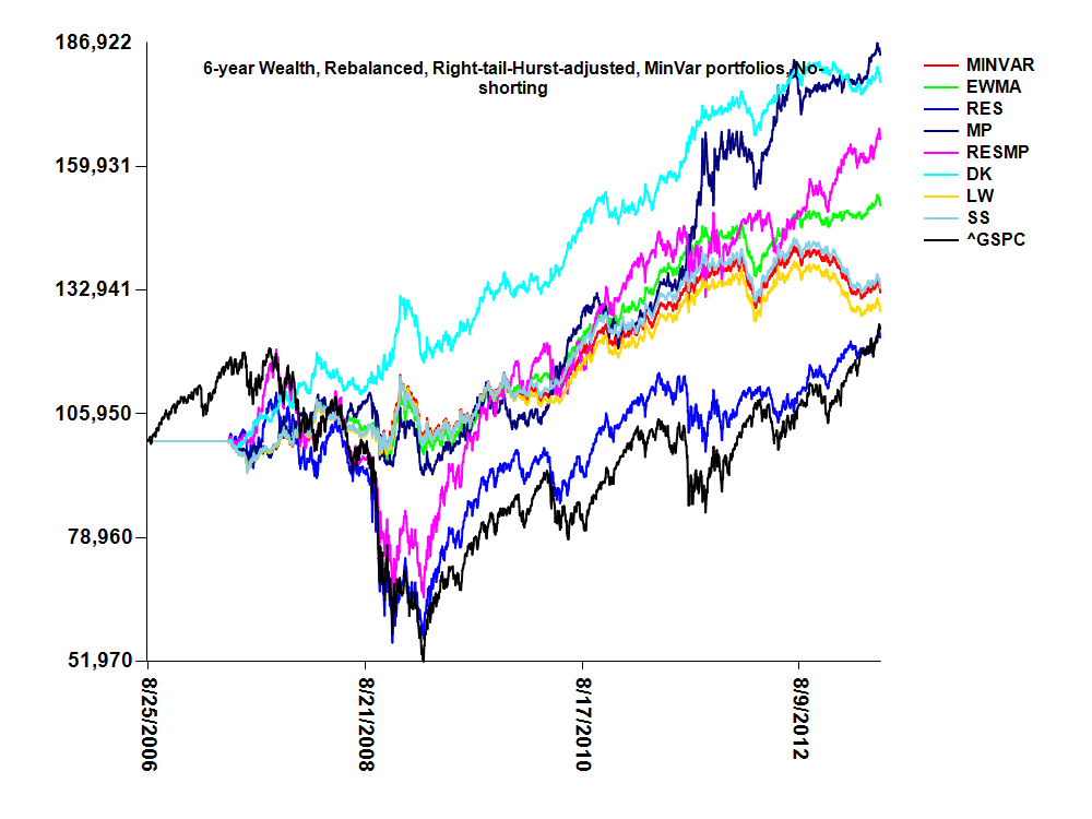
C for these assets, eight types of portfolios was constructed, five of which involved transformations applied to the log-return data (MinVar, EWMA, RES, MP, RESMP) and three types which involved covariance matrix "shrinkage" methods (DK, LW, and SS). Covariance matrix shrinkage techniques attempt to reduce the covariance matrix to an identity matrix. Recall, the more a covariance matrix is like an identity matrix, the more homogeneous the eigenvalues, since if the covariance matrix is truly an identity matrix,
R=
I, and all of its eigenvalues will be one. This follows the property that the determinant of an identity matrix
I is one, since the product of all of its eigenvalues, Πλ, is unity. The MinVar portfolio is a Markowitzian minimum variance portfolio (not tangency). The EWMA portfolio uses an exponential weighted moving average determination of returns and their standard deviations. The RES approach employs "component subtraction" (see
Chap 28) to remove the effect of the first principal component (eigenvector) of the correlation matrix on returns. (this is also known as removing the "market" effect from returns, since the eigenvector of
R associated with the greatest eigenvalue typically reflects widespread market correlations. The MP, or Marčenko-Pastur technique, uses component subtraction to remove the effect of noise eigenvectors (whose λ<λ+) on returns. The RESMP approach includes component subtraction to remove effects of both the principal eigenvector and noise eigenvectors below the MP cutoff. Lastly, the DK (Daniels-Kass), LW (Ledoit-Wolf), and SS (Schäfer-Strimmer) methods focus on various covariance matrix "shrinkage" methods, which attempt to [i] stabilize
R by forcing it to be positive definite with non-zero eigenvalues, [ii] become well-conditioned so that the ratio of the largest to the smallest eigenvalue is not too large, and [iii] reduce variance related to bias-variance decomposition. All portfolios included dividends, and did not involve tangency weights, but rather the minvar weights. Portfolio weights were determined quarterly using a 60 trading-day (3 months with 20 trading days per month) testing period and historical 180-day training period. Portfolio weights after each rebalance were also adjusted by multiplying each weight by one minus the tail probability (significance test p-value) for testing that the right-tail slope is greater than the left slope [when abs(log-return) was regressed on percentiles of log-returns] and also by multiplying the previously adjusted weights by the asset's 96-day Hurst exponent. No shorting was allowed, and weights were always constrained to sum to unity after each adjustment. Portfolio rebalancing involved purchase of assets according to the weights, using all existing proceeds in the portfolio. The 6-year wealth plot below shows results for the eight portfolios after an initial $100,000 investment during the first rebalance using the adjusted weights obtained. For comparison purposes, an initial purchase of $100,000 was made in the S&P500 index (^GSPC from Yahoo), which remained unbalanced. For a quarterly rebalance, the DK shrinkage portfolio resulted in approximately $180k 6 years after April 30, 2007.
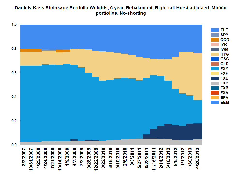
A chart of the rebalance-specific weights for the 6-year quarterly-rebalanced DK shrinkage portfolio is shown below, where the most recent non-zero weights for the last rebalance period (May 1, 2013) were HYG(48.8%), TLT(20.7%), FXY(17.5%), FXE(7.8%), FXC(4.5%), and IYR(0.7%). (weights for other portfolios using different adjustments and time frames are provided
here). Note that this is a hedging portfolio focusing on asset preservation. That weights were adjusted for right-tail events may minimize exposure to assets with left-tail ("black-swan") dominance. Adjusting weights at each rebalance by the epoch-specific historical 96-day Hurst exponent provides more weight for assets with greater stability.

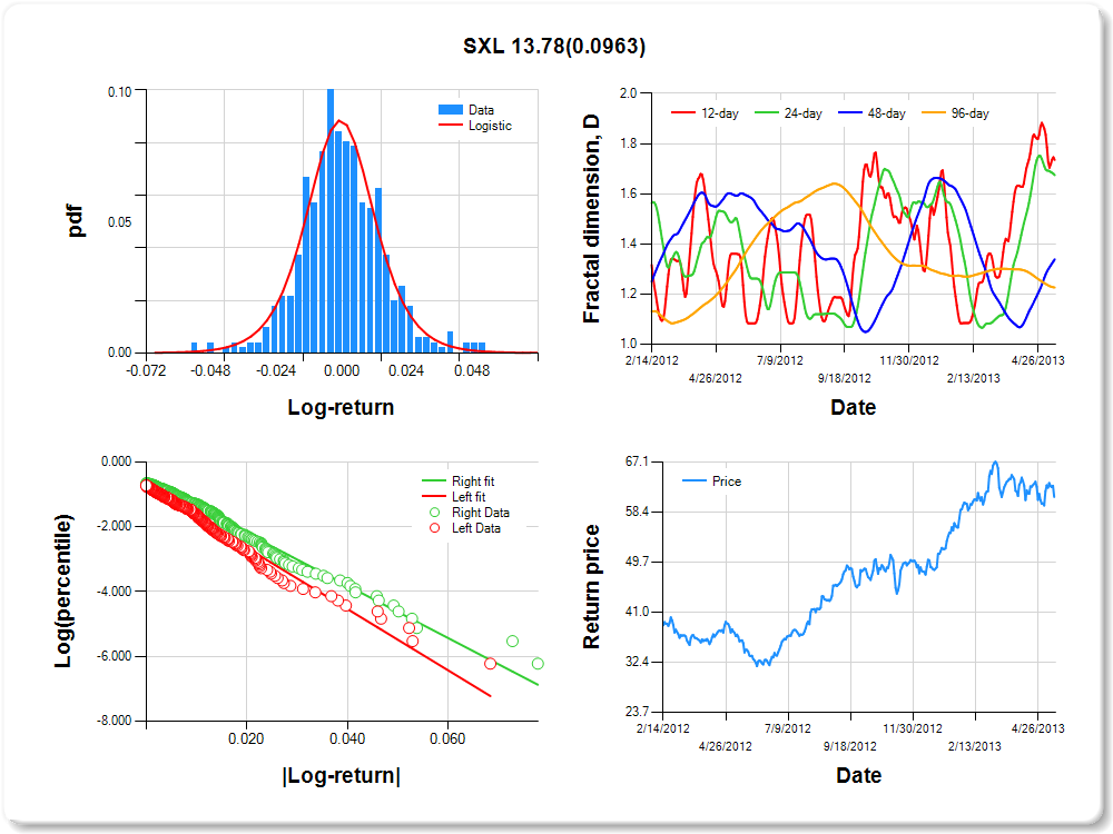
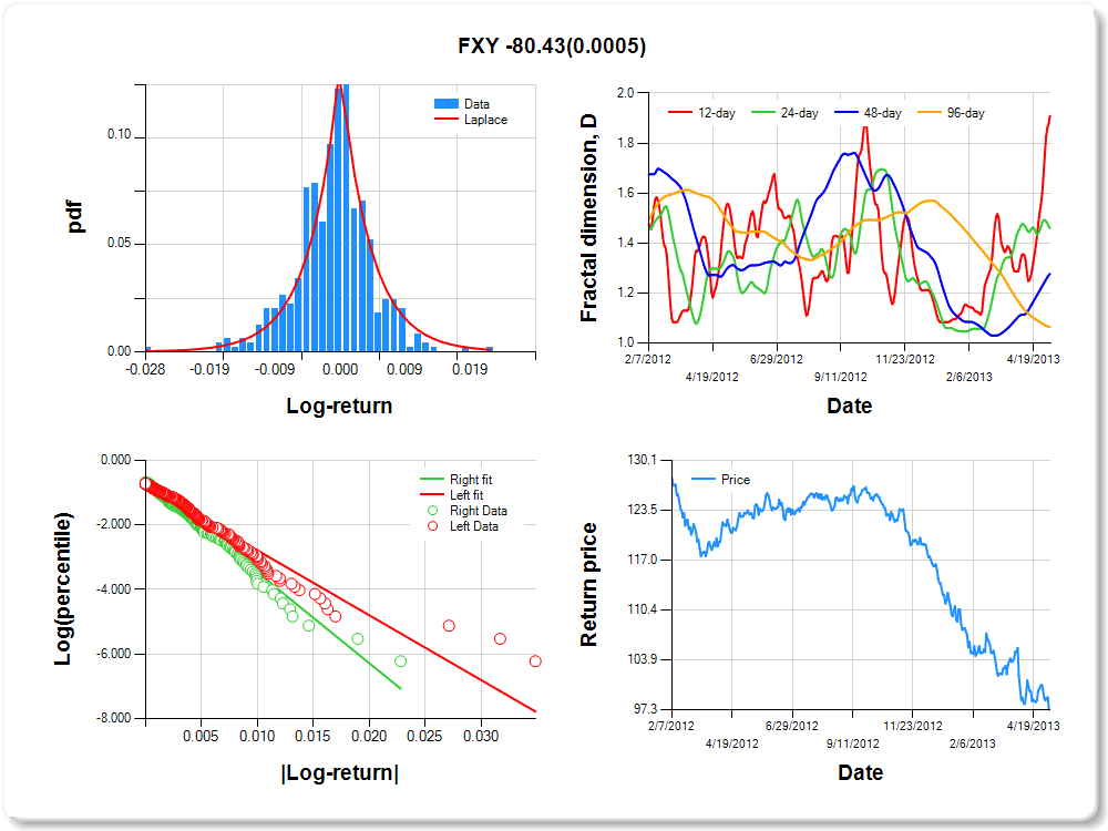
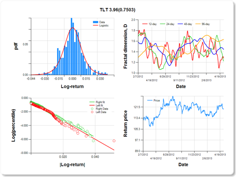
Regarding risk and stability of assets considered for portfolio input, the chart below shows an example of a 2-year historical summary of an asset [Sunoco Logistics (
SXL)] whose price returns are more right-tail dominant and stable. In the upper left panel, it can be readily observed that the frequency of occurrence of log-returns is greater in the right tail. This was verified quantitatively by regressing abs(log-return) on percentiles, for which the slope for right tail returns was significantly greater than the slope for left tail returns (slope of green fitted line vs. red fitted line). The regression coefficient for a test of equal slopes (13.78) is listed in the chart title, along with the significance level, which is important but not less than 0.05. The upper right panel shows the 12-, 24-, 48-, and 96-day fractal dimension,
D, which by definition fall in the range [1,2]. Values of
D near 1 suggest high stability, whereas values approaching 2 suggest instability. Since the Hurst exponent,
H, is equal to 2-
D, values in the range 0.5<
H<1 are termed "persistent" (like the frequency of ocean waves), whereas values of 0<
H<0.5 are "anti-persistent," similar to fractal Brownian processes. Persistent time series processes tend to go up after a previous increase and down after a previous decrease, which is not true for anti-persistent time series. On May 1, 2013, SXL had a low 96-day
D near 1.2, and therefore, over longer periods, SXL tended to be stable. Recently, however, the 12-, 24-, and 48-day
D's for SXL are picking up, suggesting that the price return time series is becoming more unstable (breaking up). This can be seen in the lower right panel, which reflects that the price return is starting to become more choppy.
Below are listed the risk and stability characteristics of the assets with non-zero weights in the quarterly-rebalanced 6-year DK portfolio, ordered by their 6-year 96-day Hurst exponents. The 2-years histories and calculations are provided to gain a better view of their price fractal dimension.
FXY-CurrencyShares Japanese Yen Trust
Percentile values of daily loss(gain) in per cent
|
0.5
|
1
|
5
|
10
|
25
|
50
|
75
|
90
|
95
|
99
|
99.5
|
-0.03
|
-0.02
|
-0.01
|
-0.01
|
0.00
|
0.00
|
0.00
|
0.01
|
0.01
|
0.01
|
2.52
|
Daily log-return distribution fitting results
|
Distribution
|
Location, a
|
Scale, b
|
Laplace
|
0.387
|
0.260
|
Linear regression results [Model: y=log(percentile of log-return), x=|log-return|]
|
Variable
|
Coef
|
s.e.
|
t-value
|
P-value
|
Constant
|
-0.774
|
0.091
|
-8.544
|
0.0000
|
|log-return|
|
-200.603
|
13.739
|
-14.601
|
0.0000
|
I(right-tail)
|
0.130
|
0.130
|
1.006
|
0.3148
|
|log-return|*I(right-tail)
|
-80.430
|
23.055
|
-3.489
|
0.0005
|
Hurst exponent (of daily return price)
|
12-day
|
24-day
|
48-day
|
96-day
|
0.091
|
0.541
|
0.723
|
0.936
|
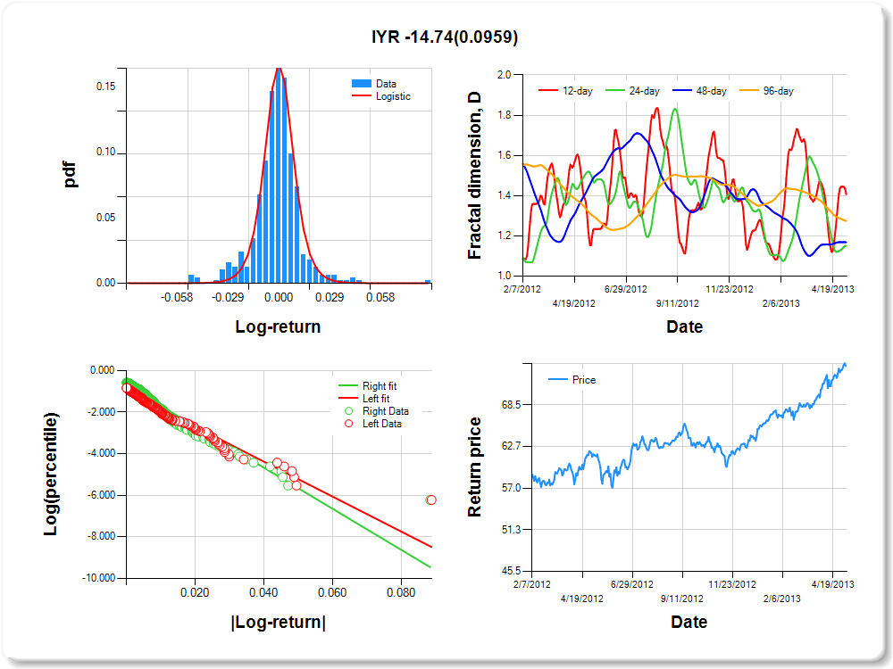
IYR- iShares Dow Jones US Real Estate ETF
Percentile values of daily loss(gain) in per cent
|
0.5
|
1
|
5
|
10
|
25
|
50
|
75
|
90
|
95
|
99
|
99.5
|
-0.05
|
-0.04
|
-0.02
|
-0.01
|
0.00
|
0.00
|
0.01
|
0.02
|
0.04
|
0.05
|
2.15
|
Daily log-return distribution fitting results
|
Distribution
|
Location, a
|
Scale, b
|
Logistic
|
0.038
|
0.102
|
Linear regression results [Model: y=log(percentile of log-return), x=|log-return|]
|
Variable
|
Coef
|
s.e.
|
t-value
|
P-value
|
Constant
|
-1.017
|
0.090
|
-11.333
|
0.0000
|
|log-return|
|
-84.104
|
6.120
|
-13.743
|
0.0000
|
I(right-tail)
|
0.301
|
0.121
|
2.487
|
0.0132
|
|log-return|*I(right-tail)
|
-14.743
|
8.838
|
-1.668
|
0.0959
|
Hurst exponent (of daily return price)
|
12-day
|
24-day
|
48-day
|
96-day
|
0.593
|
0.850
|
0.832
|
0.726
|
HYG-iShares iBoxx $ High Yid Corp Bond
Percentile values of daily loss(gain) in per cent
|
0.5
|
1
|
5
|
10
|
25
|
50
|
75
|
90
|
95
|
99
|
99.5
|
-0.02
|
-0.02
|
-0.01
|
0.00
|
0.00
|
0.00
|
0.00
|
0.01
|
0.02
|
0.02
|
2.69
|
Daily log-return distribution fitting results
|
Distribution
|
Location, a
|
Scale, b
|
Laplace
|
0.326
|
0.184
|
Linear regression results [Model: y=log(percentile of log-return), x=|log-return|]
|
Variable
|
Coef
|
s.e.
|
t-value
|
P-value
|
Constant
|
-1.062
|
0.086
|
-12.336
|
0.0000
|
|log-return|
|
-181.256
|
13.254
|
-13.676
|
0.0000
|
I(right-tail)
|
0.407
|
0.122
|
3.346
|
0.0009
|
|log-return|*I(right-tail)
|
-29.503
|
18.858
|
-1.565
|
0.1183
|
Hurst exponent (of daily return price)
|
12-day
|
24-day
|
48-day
|
96-day
|
0.807
|
0.863
|
0.628
|
0.665
|
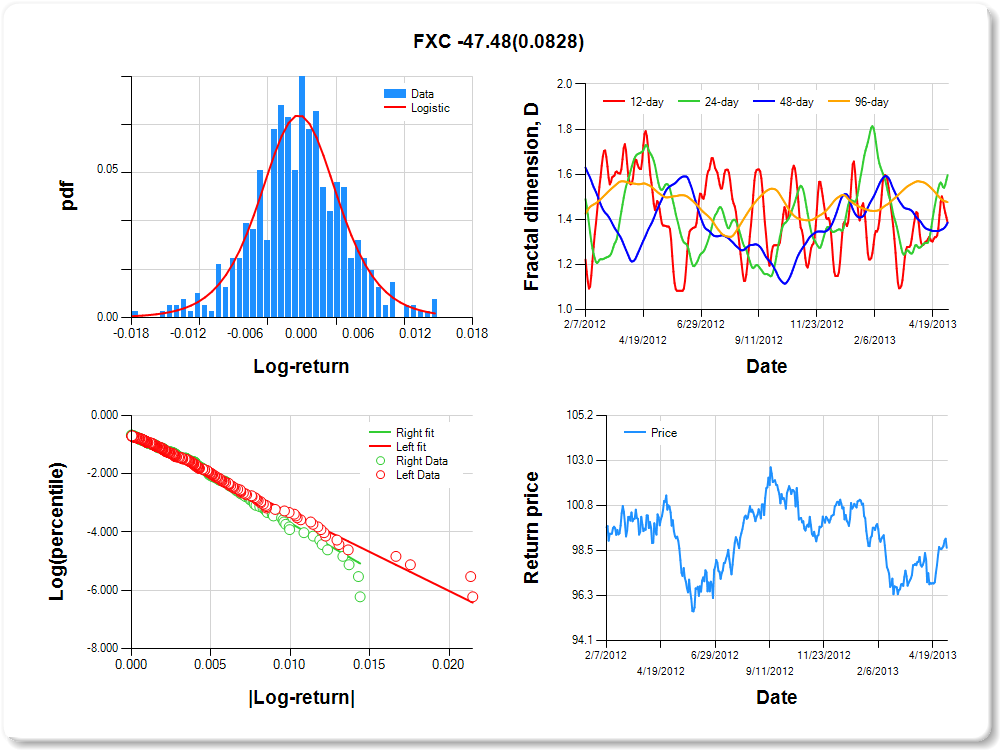
FXC-CurrencyShares Canadian Dollar Trust
Percentile values of daily loss(gain) in per cent
|
0.5
|
1
|
5
|
10
|
25
|
50
|
75
|
90
|
95
|
99
|
99.5
|
-0.02
|
-0.01
|
-0.01
|
-0.01
|
0.00
|
0.00
|
0.00
|
0.01
|
0.01
|
0.01
|
5.88
|
Daily log-return distribution fitting results
|
Distribution
|
Location, a
|
Scale, b
|
Logistic
|
0.340
|
0.253
|
Linear regression results [Model: y=log(percentile of log-return), x=|log-return|]
|
Variable
|
Coef
|
s.e.
|
t-value
|
P-value
|
Constant
|
-0.649
|
0.094
|
-6.911
|
0.0000
|
|log-return|
|
-268.174
|
17.793
|
-15.072
|
0.0000
|
I(right-tail)
|
0.129
|
0.136
|
0.952
|
0.3417
|
|log-return|*I(right-tail)
|
-47.485
|
27.319
|
-1.738
|
0.0828
|
Hurst exponent (of daily return price)
|
12-day
|
24-day
|
48-day
|
96-day
|
0.615
|
0.404
|
0.614
|
0.524
|
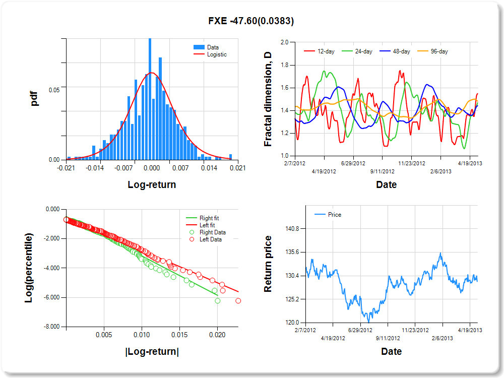
FXE-CurrencyShares Euro Trust
Percentile values of daily loss(gain) in per cent
|
0.5
|
1
|
5
|
10
|
25
|
50
|
75
|
90
|
95
|
99
|
99.5
|
-0.02
|
-0.02
|
-0.01
|
-0.01
|
0.00
|
0.00
|
0.00
|
0.01
|
0.01
|
0.02
|
4.38
|
Daily log-return distribution fitting results
|
Distribution
|
Location, a
|
Scale, b
|
Logistic
|
0.129
|
0.275
|
Linear regression results [Model: y=log(percentile of log-return), x=|log-return|]
|
Variable
|
Coef
|
s.e.
|
t-value
|
P-value
|
Constant
|
-0.589
|
0.097
|
-6.099
|
0.0000
|
|log-return|
|
-219.984
|
14.582
|
-15.086
|
0.0000
|
I(right-tail)
|
0.106
|
0.140
|
0.759
|
0.4483
|
|log-return|*I(right-tail)
|
-47.599
|
22.919
|
-2.077
|
0.0383
|
Hurst exponent (of daily return price)
|
12-day
|
24-day
|
48-day
|
96-day
|
0.450
|
0.531
|
0.557
|
0.518
|
TLT-iShares Barclays 20+ Yr Treas.Bond
Percentile values of daily loss(gain) in per cent
|
0.5
|
1
|
5
|
10
|
25
|
50
|
75
|
90
|
95
|
99
|
99.5
|
-0.03
|
-0.03
|
-0.02
|
-0.01
|
-0.01
|
0.00
|
0.01
|
0.02
|
0.03
|
0.04
|
3.36
|
Daily log-return distribution fitting results
|
Distribution
|
Location, a
|
Scale, b
|
Logistic
|
0.283
|
0.221
|
Linear regression results [Model: y=log(percentile of log-return), x=|log-return|]
|
Variable
|
Coef
|
s.e.
|
t-value
|
P-value
|
Constant
|
-0.654
|
0.102
|
-6.395
|
0.0000
|
|log-return|
|
-133.370
|
9.356
|
-14.255
|
0.0000
|
I(right-tail)
|
0.134
|
0.137
|
0.980
|
0.3273
|
|log-return|*I(right-tail)
|
3.957
|
12.427
|
0.318
|
0.7503
|
Hurst exponent (of daily return price)
|
12-day
|
24-day
|
48-day
|
96-day
|
0.718
|
0.774
|
0.557
|
0.368
|
Before considering assets for portfolio construction, it is helpful to characterize whether the log-return distribution is left or right tail dominant, and how persistent the price return time series is. Certainly, the fundamentals concerning valuation, surprises in future earnings growth, economic moat, and shocks from geopolitical or legal events may drastically change price return characteristics. As usual, there are other ways to study risk and stability of times series; however, emphasis on right-tail dominance and greater Hurst exponents may minimize risk and increase stability in the near term. Additional unbalanced and quarterly-rebalanced 2-,5-, and 10-year portfolios for the Dow 30, Vanguard Funds, Fidelity Funds, dividend assets, volatilty (collar) assets, commodities, sector ETFs, and gold stocks are provided at
RandomMatrixPortfolios. Readers interested in detailed algorithms and computational aspects of correlation and covariance matrices, eigendecomposition, the Marčenko-Pastur limit distribution of eigenvalues for a random matrix, component subtraction for the RES, MP, and RESMP methods, and covariance matrix shrinkage techniques can refer to chapters
12 and
28 of a new book on machine learning and computational intelligence approaches to pattern discovery and classification.
Disclosure: I have no positions in any stocks mentioned, and no plans to initiate any positions within the next 72 hours. I wrote this article myself, and it expresses my own opinions. I am not receiving compensation for it (other than from Seeking Alpha). I have no business relationship with any company whose stock is mentioned in this article.